Why value bridges need an equity dilution or concentration value driver

Private equity value creation models should include a value driver that measures gains or losses driven by changes in the Fund or GP’s share of company (equity dilution or equity concentration).

Here’s why…

 

 

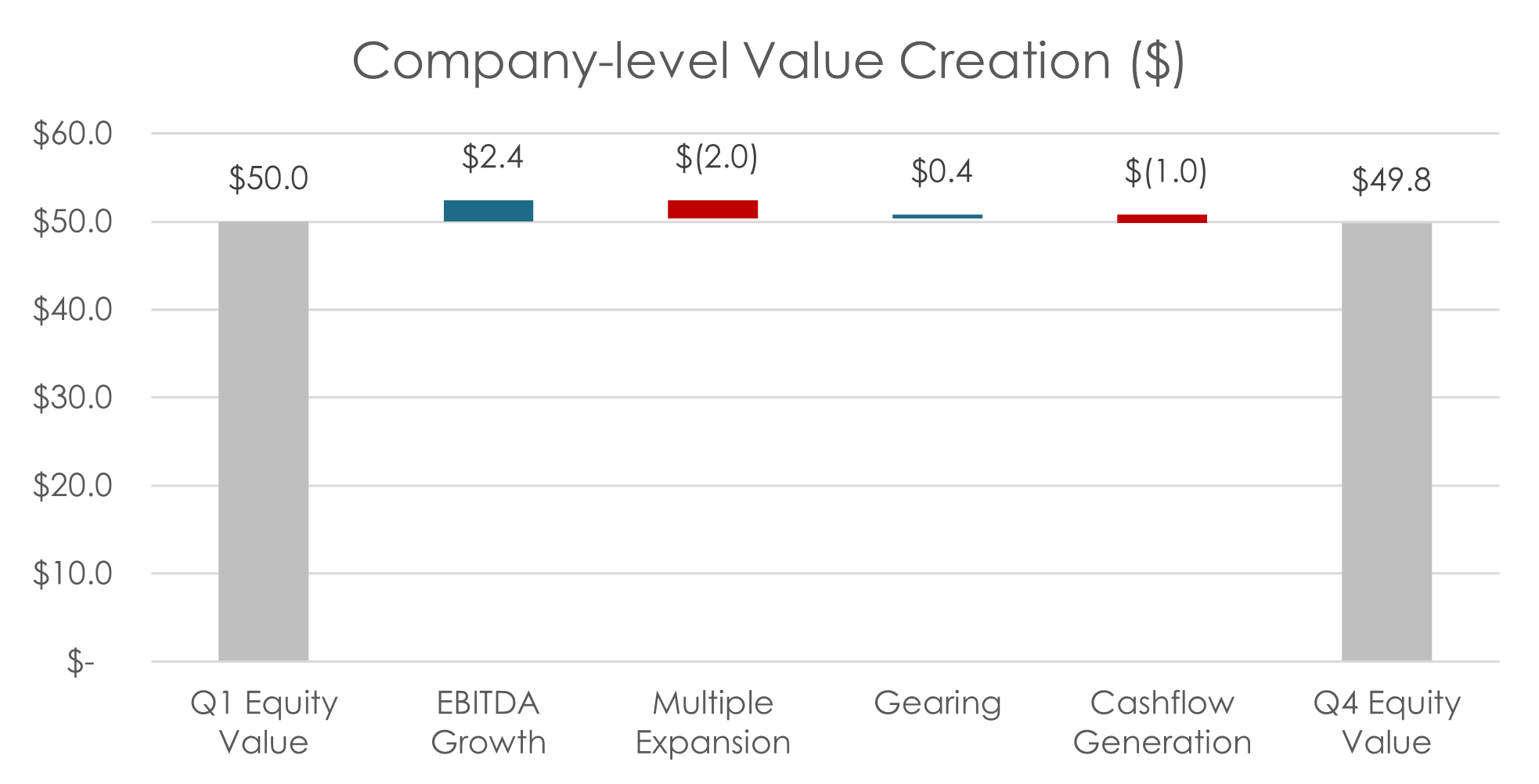
The following table provides capital structure and income statement data for a private equity deal. It is a $100 million company with $50 million of debt and $50 million of equity. As of Q1, the company has TTM EBITDA of $20 million, so its enterprise valuation multiple is 5.00x.

		Q1	Q4		ΔX	Avg. X
	Total Equity (TEqV)	$50.0	$49.8		-$0.2	$49.9
	Net Debt (ND)	$50.0	$51.0		+$1.0	–
	Enterprise Value (TEV)	$100.0	$100.8		+$0.8	$100.4
	Equity Ratio (ER)	50.0%	49.4%		-0.6%	49.7%
	Debt Ratio (DR)	50.0%	50.6%		+0.6%	50.3%
	EBITDA (E)	$20.0	$21.0		+$1.0	$20.5
	Valuation Multiple (M)	5.00x	4.80x		-0.20x	4.90x
	Fund Equity (FEqV)	$30.0	$31.0		+$1.0	–
	Fund Ownership (φ)	60.0%	62.2%		+2.2%	61.1%

Over the next few quarters, the numbers change a bit. TTM EBTIDA increases to $21 million, but market comps are down, so the valuation multiple decreases to 4.80x. Also, the company burns through $1.0 million of cash, so its net debt is $51.0 million. This provides a Q4 enterprise valuation of $100.4, a total equity valuation of $49.8, and slight changes in equity and debt ratios.

Even though the total equity change is only -$200 thousand, the underlying value drivers are more substantial. At the company level, the sources of total equity value creation are EBITDA Growth (V_EG), Multiple Expansion (V_ME), Gearing (V_GEAR), and Cashflow Generation (V_CF).

   

   

   

   

These four value drivers sum to the total equity loss of -$200 thousand, and bridge the gap between the Q1 equity value of $50.0 million and the Q4 equity value of $49.8 million.

 

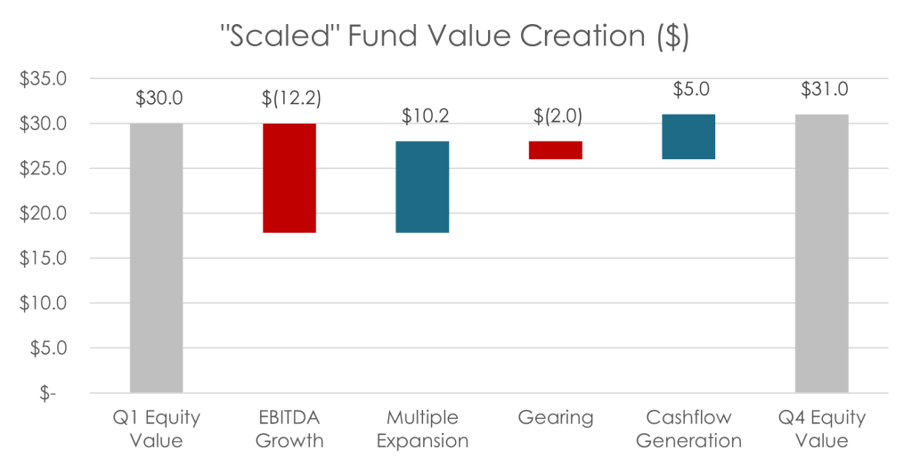
Investors are typically concerned with the returns of a specific shareholder, like a Fund or GP. In this deal, the GP’s equity value increases from $30.0 million to $31.0 million. GPs can sometimes outperform other shareholders, as above, when they use structure, like participating preferred securities.

 

How should we translate company-wide value drivers to Fund or GP value drivers?

One approach that *sometimes* works is to multiply the value drivers by the change in Fund Equity (ΔFEqV) and then divide by the change in Total Equity (ΔTEqV), as follows:

   

   

   

   

However, this is an example where this approach *does not* work. It flips the value drivers in the wrong direction and amplifies values to be much larger than what should be expected from the small changes on the company’s income statement and balance sheet.

 

To fix this, we must bring the Fund Ownership (φ) into the model. Multiply the four value drivers by the average holding period Fund Ownership of 61.1%.

   

   

   

   

Now the value drivers have the correct sign and magnitude, but they do not bridge the gap between the Q1 Fund Equity of $30.0 and Q4 Fund Equity of $31.0. We must include Fund Ownership Impact (V_FO), which measures equity value creation driven by increasing ownership (equity concentration) or decreasing ownership (equity dilution).

   

   

Adding V_FO to the chart completes the value bridge:

 

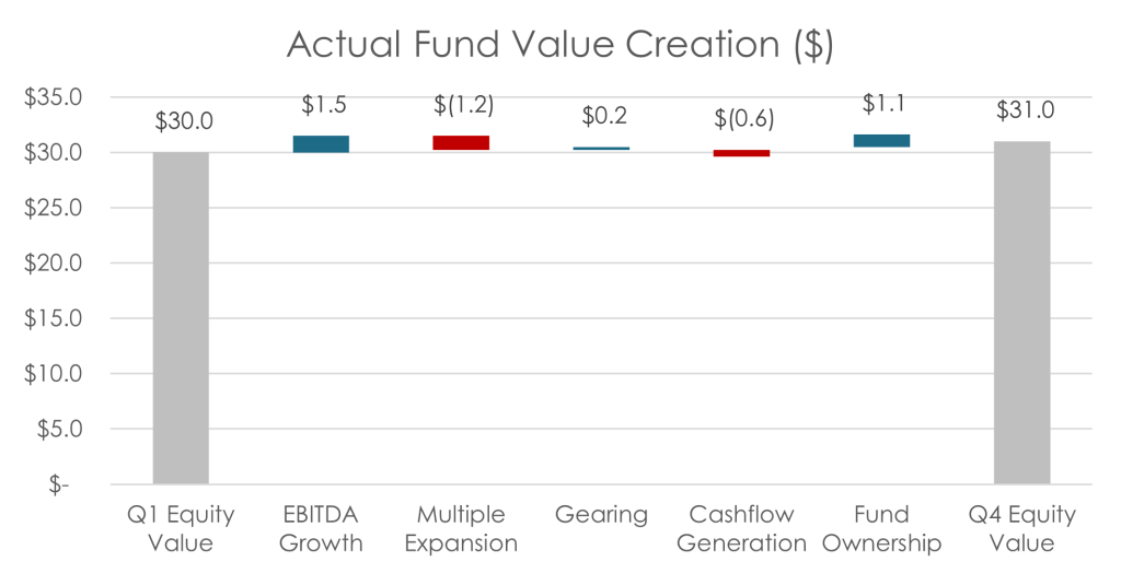
These value drivers match what should be expected from intuition: GP equity value increases from slightly growing TTM EBITDA and enterprise valuation, which are offset by contracting valuation multiples and burning cash. Without an increase in ownership, the GP’s equity would have decreased by 0.4%.

However, structure allows the GP to increase φ, create $1.1 million of additional equity value, an increase the value of its investment to $31.0 million.